Local Synapse Snapshots

This vignette explains how to use a local copy of the Aedes synapse table to enable connectivity queries that can reflect edits up to the latest second but are still very fast (think one second to find the partners of hundreds of neurons vs 5 minutes via CAVE). The catch is a one time download of about 2 GB of data onto the user’s machine. You also have access to the full synapse table including the location of every synapse.

Quick Start

If you have access to the aedes CAVE datastack:

library(aedes)
aedes_use_snapshot()
aedes_set_version('now')
dn.now <- aedes_partner_summary("superclass:descending_neuron", partners = "inputs")
aedes_set_version('latest')
dn.lat <- aedes_partner_summary("superclass:descending_neuron", partners = "inputs")

The first time, aedes_use_snapshot() offers to download a snapshot (consisting of about 1.6 GB of static synapse data (e.g. XYZ locations) that never changes and 0.5 GB of materialisation information that matches each row of that synapse table to current root_ids). After that, new checkpoints (a few MB) are downloaded automatically every day when you use the snapshot and deltas up to the current time can be computed on your machine. Collectively this allows rapid time travel to arbitrary timepoints in the evolving connectome connectivity graph. In particular this allows users to access both the latest CAVE materialisation version (e.g. 519) and the current time ("now") for up-to-the-second queries. We find this very useful during simultaneous proofreading and typing.

Key Points

• Snapshots are made on a lab server and downloaded automatically: one full base, plus a small checkpoint each day at each materialisation version.
• For "now", or any time after the latest snapshot, aedes fetches the edits made since that snapshot from CAVE. The result is kept in memory for the rest of the R session, so only the first query is slow. Nothing is written to disk.
• Root ids only make sense at one time, so fix the time once (now <- Sys.time()) and use it for every call in an analysis block.
• Each materialisation version has its own snapshot (e.g. v519), so repeating an analysis at a version needs no CAVE lookups.

Read on for more details, and see Handling recent edits for how times after the newest snapshot work.

Introduction

How a local snapshot is used alongside CAVE

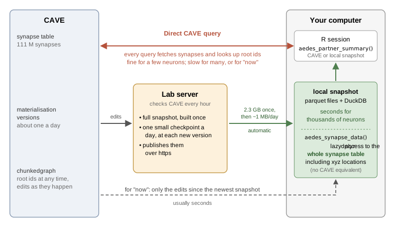
The Aedes synapse table has about 111 million synapses. Querying it through CAVE is fine for a few neurons, but it is slow for tens to thousands of neurons, especially at the latest state of the dataset. A local synapse snapshot is a copy of the whole table as parquet files, which aedes queries with DuckDB. This gives you:

• fast queries for the latest state of the dataset (“now”). Only the edits made since the snapshot are fetched from CAVE, so you can work with up to date connectivity for large numbers of neurons. This is impractical with live CAVE queries.
• fast partner summaries. Thousands of neurons take seconds.
• the full synapse table, including the positions of the pre and postsynaptic points and the synapse size, for your own dplyr queries with aedes_synapse_data(). The root_ids can be at any time including “now”. Only needs the standard downloaded snapshot. Although it is possible to download the whole synapse table from CAVE at a specific materialisation version, it takes about an hour multi-threaded and the devs will not like it if you make a habit of this.
• a fast local cache of a materialisation version. CAVE (via the chunkedgraph) already lets you go back to any time; a snapshot makes repeating an analysis at one particular version fast.

Vocabulary

Term	Meaning
synapse table	the CAVE table with every synapse in the dataset
static data	the columns of the synapse table that never change: synapse id, pre and postsynaptic supervoxels, positions and size (static.parquet, 1.6 GB)
snapshot	the root ids of both partners of every synapse at one moment in time, named by a tag such as v518
base	a full snapshot (0.55 GB), usually at a CAVE materialisation version
checkpoint	a snapshot stored as just the synapses whose root ids changed since an earlier snapshot, its parent (about 1 MB per day of edits)

Who Does What

Most people only use snapshots:

• download them with aedes_download_snapshot()
• use them with aedes_use_snapshot(), aedes_partner_summary() and aedes_synapse_data()
• update them to a later time with aedes_update_snapshot() (or just download again)

Someone looking after the snapshots (for now on a lab server) does the rest:

• build the static data and a first base with aedes_build_snapshot()
• make daily checkpoints and occasional new bases with a cron job (inst/scripts/synsnap-cron.sh)
• distribute them with aedes_publish_snapshot()

Using a Snapshot

You select a snapshot once per session. The snapshot folder is found by aedes_snapshot_root().

library(aedes)
library(dplyr)
aedes_use_snapshot()
#> Using synapse snapshot 'r20261001T200000' (2026-10-01 20:00:00 UTC)

aedes_use_snapshot() respects the version you have chosen for other aedes functions (see aedes_set_version()). By default this is "now" (the package says so when it loads), so you get the newest snapshot, which is then brought up to the present on the fly. With aedes_set_version("latest") you get the snapshot made at the newest CAVE materialisation version instead. You can also ask for a specific version or timestamp; this also changes the default for the other aedes functions so that metadata and connectivity match.

aedes_use_snapshot(timestamp = "now")
aedes_use_snapshot(version = 519)

Partner summaries are now answered locally:

aedes_partner_summary("superclass:descending_neuron", partners = "inputs")

You can ask about later times than the snapshot, including timestamp = "now". In this case aedes_partner_summary() fetches just the edits made since the newest snapshot from CAVE and looks up new root ids for the synapses that they affect. The update is kept for the rest of the session, so only the first query after a long gap is slow.

aedes_partner_summary("superclass:descending_neuron", partners = "inputs",
                      timestamp = "now")

For anything else, aedes_synapse_data() gives you a lazy table of every synapse that works with dplyr verbs. Unlike aedes_partner_summary(), which falls back to CAVE, it needs a local snapshot. Nothing is actually read until you collect() the result. For example to count the inputs onto descending neurons by presynaptic partner:

dns <- aedes_ids("superclass:descending_neuron")
aedes_synapse_data("post") %>%
  filter(post_root %in% dns) %>%
  count(pre_root, sort = TRUE) %>%
  collect()

Root ids come back as integer64 columns, but you can filter with the character ids that aedes_ids() returns. With details = TRUE the table also has supervoxel ids, the positions of the pre and postsynaptic points and the synapse size.

Synapses at a Particular Time

By default aedes_synapse_data() reads the selected snapshot exactly as it is. To get the synapses at another time, give timestamp. This works just like aedes_partner_summary(): the edits since the newest snapshot are looked up in CAVE and kept in memory. So the result only works in the current R session; collect() it there.

Root ids only mean something at one time, so look up the neurons you are interested in at the same time as the synapses. Fixing the time once makes sure that they match:

now <- Sys.time()
dns <- aedes_ids("superclass:descending_neuron", timestamp = now)
aedes_synapse_data("post", timestamp = now) %>%
  filter(post_root %in% dns) %>%
  count(pre_root, sort = TRUE) %>%
  collect()

Repeating an Analysis at a Materialisation Version

Each materialisation version has its own snapshot, named v<version>. You can repeat an analysis at that version exactly, with no CAVE lookups for the synapses:

dns519 <- aedes_ids("superclass:descending_neuron", version = 519)
aedes_synapse_data("post", snapshot = "v519") %>%
  filter(post_root %in% dns519) %>%
  count(pre_root, sort = TRUE) %>%
  collect()

Synapse Positions

With details = TRUE you can get the location and size of each synapse. For example, here are the output synapses of one descending neuron, placed midway between the pre and postsynaptic points (in raw voxel coordinates):

aedes_synapse_data(details = TRUE, timestamp = now) %>%
  filter(pre_root %in% !!dns[1]) %>%
  mutate(x = (pre_x + post_x) / 2, y = (pre_y + post_y) / 2,
         z = (pre_z + post_z) / 2) %>%
  select(id, post_root, x, y, z, size) %>%
  collect()

Note the !! in filter(). dplyr translates the code inside filter() into SQL, so dns[1] would otherwise be turned into an SQL expression instead of being evaluated in R; !! evaluates it in R first and inserts the result. You don’t need it for a plain variable like dns.

Assigning Synapses to Brain Regions

Synapse positions can be combined with meshes to work out where each synapse is. For example, which descending neurons get the most input in the optic lobes? The aedes_ol_meshes neuroglancer layer has meshes for the central brain (CB), each optic lobe (OL_L, OL_R) and their neuropils. They are stored in neuroglancer’s legacy precomputed format, which we can read with a small helper using code from the malevnc package:

read_ol_meshes <- function(names, base = "https://flyemdev.mrc-lmb.cam.ac.uk/flyconnectome/rclone/aedes_ol_meshes") {
  sp <- jsonlite::fromJSON(file.path(base, "segment_properties/info"))
  ids <- setNames(sp$inline$ids, sp$inline$properties$values[[1]])
  bad <- setdiff(names, names(ids))
  if (length(bad)) stop("Unknown mesh name(s): ", toString(bad),
                        ". Choose from: ", toString(names(ids)))
  lapply(ids[names], \(id) {
    frags <- jsonlite::fromJSON(paste0(base, "/", id, ":0"))$fragments
    Reduce(merge, lapply(file.path(base, frags), malevnc:::read_neuroglancer_mesh))
  })
}
meshes <- read_ol_meshes(c("CB", "OL_L", "OL_R"))

Now fetch the position of every input synapse onto the descending neurons and test which mesh each one is inside. Synapse positions are in raw voxels, but the meshes are in nm, so convert with aedes_raw2nm() first:

syn <- aedes_synapse_data(details = TRUE, timestamp = now) %>%
  filter(post_root %in% dns) %>%
  select(id, pre_root, post_root, post_x, post_y, post_z) %>%
  collect()
xyz <- aedes_raw2nm(as.matrix(select(syn, post_x, post_y, post_z)))
inside <- as_tibble(lapply(meshes, \(m) nat::pointsinside(xyz, m)))

This takes a couple of seconds for about 1.5 million synapses. Then count the synapses in each region for each neuron. A few synapses are outside all three meshes and are counted as other:

dn_regions <- syn %>%
  bind_cols(inside) %>%
  mutate(region = case_when(CB ~ "CB", OL_L ~ "OL_L", OL_R ~ "OL_R",
                            .default = "other")) %>%
  count(post_root, region) %>%
  tidyr::pivot_wider(names_from = region, values_from = n, values_fill = 0) %>%
  mutate(OL = OL_L + OL_R, OL_vs_CB = OL / CB)

dn_regions %>%
  slice_max(OL_vs_CB, n = 4)

Almost all descending neuron input is in the central brain: only a handful of neurons get any input in the optic lobes, and each from one side only. Use count(pre_root, region) instead to summarise by presynaptic partner.

Comparing Two Times

Synapse ids never change, so you can join snapshots from different times by id. For example, this finds the input synapses onto descending neurons whose presynaptic neuron has been edited since version 519:

old <- aedes_synapse_data(snapshot = "v519") %>%
  select(id, old_pre = pre_root)
aedes_synapse_data("post", timestamp = now) %>%
  filter(post_root %in% dns) %>%
  inner_join(old, by = "id") %>%
  filter(pre_root != old_pre) %>%
  count(pre_root, sort = TRUE) %>%
  collect()

A new root id means the neuron was edited, not necessarily that the synapse now belongs to a different neuron.

Getting a Snapshot

aedes_download_snapshot() reads a manifest.json from the server where the snapshots are published (working out its address needs access to the aedes CAVE datastack) and downloads any snapshots that you don’t have yet, into aedes_snapshot_root(). Every file is checked against its md5 and the download resumes after an interruption, so if anything goes wrong just run it again. Snapshots never change once made, so a later download only fetches new ones: normally a few small checkpoints, and occasionally a new base.

aedes_use_snapshot() and queries for times after the chosen snapshot check for new checkpoints at most every 6 hours (set the aedes.snapshot_check_hours option to change this, or Inf to turn it off) and download them quietly. Failures are only reported once they have lasted a day.

You rarely need to make a snapshot yourself, since queries for later times work without one. But you can keep the synapses at one time on disk for later sessions (e.g. the now of an analysis you want to repeat):

aedes_update_snapshot()
#> Updating synapse snapshot 'v518' (2026-09-30 14:12:29 UTC) to
#> 2026-10-01 12:00:00 UTC (now)

This writes a local checkpoint, which takes seconds to minutes. Use aedes_update_snapshot("latest") for the time of the newest materialisation version instead. A local checkpoint is only used when you ask for exactly its time (see Handling recent edits).

Handling recent edits

You don’t need this section to use snapshots, but it explains what happens for times after the newest snapshot.

Times After the Newest Snapshot

For a time after the newest snapshot, aedes starts from the newest published snapshot and makes a small table in memory of the synapses on neurons edited since then, with their root ids at that time. Together these give the synapses at that time.

Answering a query for a time after the newest snapshot

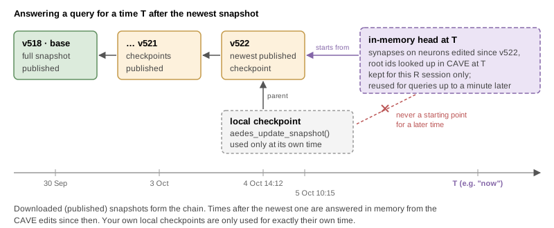
aedes_partner_summary() keeps one of these tables and moves it forward with each later query, so it only fetches the edits since the last one. aedes_synapse_data(timestamp =) keeps one table for each time you ask for. These never change, so a lazy table gives the same answer whenever you collect() it, but each new time (more than a minute after the last one, the aedes.synapse_max_age option) adds another table to the session.

Local checkpoints made with aedes_update_snapshot() are only used for exactly their own time. Later times always start from a published snapshot, for the reason below.

Edits That Become Visible Late

CAVE lists each edit with the time it was made, but it can take a little while (usually seconds, occasionally minutes) before the edit is listed. So reading the edits up to a very recent time can miss some, and anything that started from that point would go on missing them.

Edits that become visible late

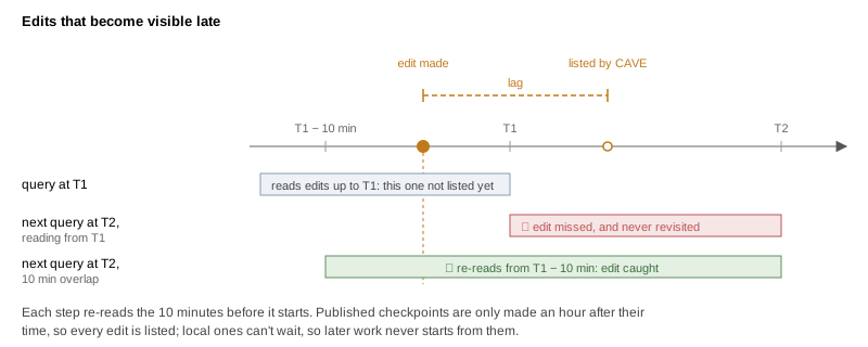
aedes avoids this in three ways:

• the lab server only makes a checkpoint an hour after its time, by which point every edit has been listed
• every update re-reads the edits from 10 minutes before the time it starts from, and edits read too soon are read again by the next query
• local checkpoints can’t wait an hour, so they are never used as a starting point

Building and Publishing Snapshots

This section is for whoever looks after the snapshots. aedes_build_snapshot() builds everything from scratch:

aedes_build_snapshot()

This does two things:

1. downloads the source edgelist behind the CAVE synapse table (22 GB), checks its md5 and converts it to static.parquet. The file is found from the description of the CAVE table, so you need access to the aedes datastack.
2. looks up the root id of every supervoxel at the newest materialisation version to make the first base, e.g. v518.

It takes a few hours and needs about 25 GB of free space while it runs, but only 2.1 GB once it has finished. If you have the Google Cloud CLI (gcloud) installed the download is quicker; otherwise curl is used. If anything goes wrong just run it again with the same version and it will carry on where it stopped. Before a new base is used, the synapses of 20 neurons of very different sizes are compared with a CAVE query at the same version. A snapshot that fails this check is moved aside rather than used.

After that, inst/scripts/synsnap-cron.sh runs hourly from cron. Each run makes any missing checkpoints from the past week: one at the exact time of each materialisation version (e.g. v519, at about 14:12 UTC), and one at 20:00 UTC on any day without a version in the 24 hours before (e.g. r20261002T200000), so there is about one a day. Each is made once an hour has passed, so that all edits are visible. It then publishes them (as aedes_publish_snapshot() does), hard linking the static data, the base and every checkpoint built on it into a folder served over https and writing manifest.json last. Finally it writes a status.json and exits with an error, so that cron sends an email, if anything failed or the newest snapshot is more than 36 hours old. A run that fails or never happens is filled in by the next one. The comments at the top of the script say how to set it up.

Reading a checkpoint gets slower as its chain back to the base grows, so every few months make a new base with aedes_update_snapshot("latest", rebase = TRUE).

How It Works

Layout

A snapshot folder holds the static data and a small folder for each snapshot:

syn_snapshot/
  static.parquet     id, pre_sv, post_sv, positions, size    1.6 GB
  static.json        source table and md5
  v518/              base
    meta.json        tag, timestamp
    by_pre.parquet   id, pre_root, post_root                 0.55 GB
  v519/              checkpoint at materialisation version 519
    meta.json        tag, timestamp, base = "v518", parent = "v518"
    log.parquet      id, t, new and old roots                about 1 MB
  r20261002T200000/  checkpoint at 20:00 (no version on 2 Oct)
    meta.json        tag, timestamp, base = "v518", parent = "v519"
    log.parquet
  v521/              checkpoint at materialisation version 521
    meta.json        tag, timestamp, base = "v518",
                     parent = "r20261002T200000"
    log.parquet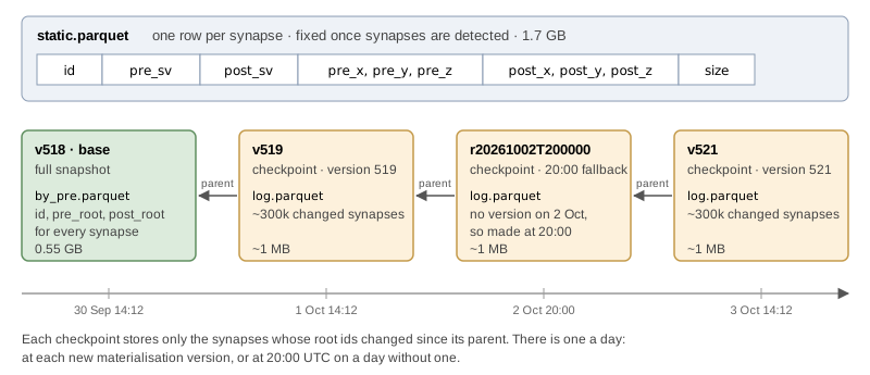

The chain of checkpoints back to the base

The split follows how the data actually change. Supervoxels, positions and sizes are fixed once synapses have been detected; proofreading only changes which root id each supervoxel belongs to. So each snapshot only stores the root ids of the two partners of each synapse, and the static columns are joined on id when you ask for them (details = TRUE).

by_pre.parquet is sorted by presynaptic root id. Parquet files store the minimum and maximum of each column for each block of rows (a row group), so DuckDB can skip most of the file when filtering on a few pre_root values. An optional copy sorted by postsynaptic root (by_post.parquet) speeds up input queries for small numbers of neurons.

Checkpoints

A checkpoint records only the synapses whose root ids changed since its parent: for each one the new root id of each side that changed, and the old one. Its parent is the newest snapshot at or before its own time, so the checkpoints form a chain back to the base. Reading a checkpoint reads the base and the logs of every checkpoint in its chain, keeping the newest root id for each synapse (below). DuckDB does this in a fraction of a second for a few neurons even with months of daily logs.

Reading a checkpoint through its chain

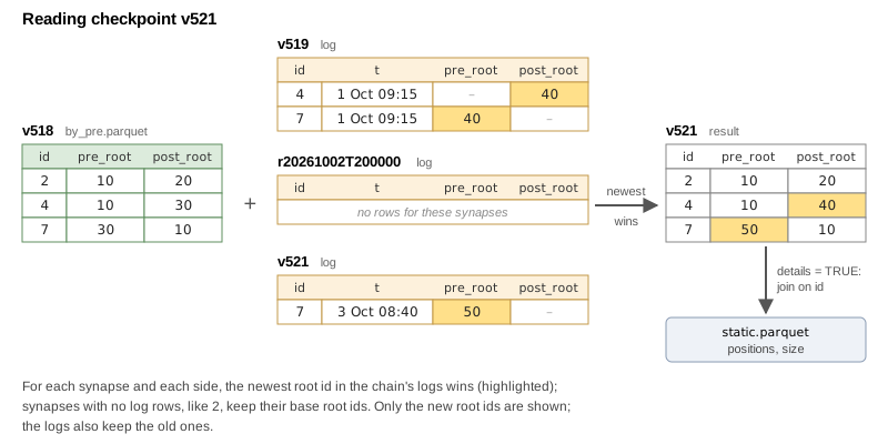
Because each checkpoint only depends on its parent, missing ones are easy to deal with:

• a missed day just makes the next checkpoint a little bigger
• a checkpoint made later for an earlier time (e.g. a day that failed and was retried later) starts a side branch from the newest snapshot before it, without changing any existing checkpoint
• a checkpoint whose chain is incomplete (e.g. a parent that failed to download) is not listed, and running the download again fills it in

Safety

• snapshots are built in .staging/ and only moved into place once they are complete and have been checked
• meta.json (for each snapshot), static.json and the published manifest.json are always the last files written
• parquet files are written to a temporary name and then renamed, so a half-written file never looks finished
• the slow steps of a build (the download and the root id lookup, which is saved in chunks of a million supervoxels) and downloads can resume after a failure

Only one process should write to a snapshot folder at a time (the cron job uses flock to make sure of this). Any number of R sessions can read from it.

Comparison with the CAVE Delta Lake Export

The CAVE materialisation engine can now export a materialisation version as a Delta Lake table (MaterializationEngine#220; see the deltalake_query notebook in CAVEColab for an example). Each version is a full copy of the synapse table, written once for each indexed column (e.g. pre and postsynaptic root id, or position) so that each copy is partitioned and sorted for queries on that column, in files of about 256 MB with extra indexes (bloom filters) to skip files quickly.

This makes it possible to query the export remotely: a client such as polars or DuckDB reads just the parts of the files it needs with HTTPS range requests, with no load on the CAVE server. This works well for a handful of neurons at a materialisation version, but gets slower when the synapses you want are spread across many files, and it can’t answer questions about the present (“now”).

	aedes snapshots	CAVE Delta Lake export
Where queries run	locally, after a download	remotely (range reads) or locally
Up front	1.6 GB static data once, plus a 0.55 GB base	nothing for remote queries
Times available	snapshot times, and “now” via CAVE edits	materialisation versions
Each new time	a checkpoint of about 1 MB per day of edits	a full copy of the table per version
Unchanged columns	stored once in static.parquet	rewritten with every version
Best for	many neurons, the latest state	a few neurons at a version, no setup

Our approach depends on two features of the synapse table:

• updates are narrow. A day of proofreading edits a few hundred neurons. Many supervoxels then belong to new root ids, but only the synapses on those neurons change, a small fraction of the 111 million rows, and the static columns are never touched. So after a one-time download of the static data and a base, each new time costs a small checkpoint.
• there is a single writer. So the only guarantee we need is that readers never see a half-built snapshot, which staging plus a rename provides.

The result is a set of ordinary parquet files that DuckDB, arrow or pandas can read directly.