Connectivity Clustering with Predicted Groups • aedes

This vignette clusters a set of related Aedes neurons by their connectivity using coconatfly’s cf_cosine_plot(). Cosine clustering compares neurons by the partners they share, and those partners must first be grouped, so that e.g. two neurons that each contact a different member of the same partner cell type still count as similar.

In well annotated datasets partners are grouped by cell type. Most aedes neurons do not yet have a type, so we compare two alternatives:

group: the curated group (see aedes_set_group()).
pgroup: the predicted group from aedes_predict_group(), which uses the first available of cell type, curated group and NBLAST cluster.

The chunks below need FlyTable and CAVE access. They are evaluated when the pkgdown website is built; elsewhere saved results are shown instead (see Rerunning this vignette).

library(aedes)
library(coconatfly)
library(dplyr)
register_aedes_coconat()

Quick start

Once register_aedes_coconat() has been called, coconatfly metadata for aedes neurons includes a pgroup column, so you can simply choose the grouping column:

cf_cosine_plot(cf_ids(aedes = "group:36155"), group = "group")
cf_cosine_plot(cf_ids(aedes = "group:36155"), group = "pgroup")

Fetch the connectivity once

As an example we use the 12 untyped visual projection neurons in group 36155. Rather than letting cf_cosine_plot() fetch connectivity each time, we fetch a connection table once with group = FALSE and then cluster it with different grouping columns.

ids <- cf_ids(aedes = "group:36155")
cf_meta(ids) %>% select(id, serial_id, side, group, nblast_group)
#>                    id serial_id side group nblast_group
#> 1  648518347546516862     36155    R 36155        36155
#> 2  648518347589781091     36156    L 36155        36155
#> 3  648518347560355394     36159    R 36155        36155
#> 4  648518347544524186     36160    R 36155        36155
#> 5  648518347553146126     36161    L 36155        36155
#> 6  648518347592422420     36164    L 36155        36155
#> 7  648518347480058719     36165    L 36155        36155
#> 8  648518347482226372     36167    R 36155        36155
#> 9  648518347513818908     36180    L 36155        36155
#> 10 648518347558714862     38437    L 36155        36155
#> 11 648518347650879288     38438    R 36155        36155
#> 12 648518347592047808     38439    R 36155        36155

x <- multi_connection_table(ids, partners = c("in", "out"), threshold = 5,
                            group = FALSE)

Partner neurons without a label in the chosen column cannot act as shared features and are dropped. We can check what fraction of the partner synapses each column covers:

cov <- x %>%
  group_by(partners) %>%
  summarise(type = sum(weight[!is.na(type)]) / sum(weight),
            group = sum(weight[!is.na(group)]) / sum(weight),
            pgroup = sum(weight[!is.na(pgroup)]) / sum(weight)) %>%
  mutate(across(-partners, ~ round(.x, 3))) %>%
  as.data.frame()
cov
#>   partners  type group pgroup
#> 1   inputs 0.002 0.161  0.161
#> 2  outputs 0.008 0.607  0.615

Cell types cover under 1% of partner synapses, so group = "type" is not useful here. Using pgroup rather than group raises coverage of output synapses from 61% to 62%. Input coverage stays low because most of the input partners are not yet in FlyTable at all.

Cluster by curated group

cf_cosine_plot(x, group = "group", labRow = "{side}_{serial_id}")
#> Warning in coconat::partner_summary2adjacency_matrix(x[["outputs"]], inputcol =
#> "pre_key", : Dropping: 1104/1715 neurons representing 11653/29629 synapses due
#> to missing ids!
#> Warning in coconat::partner_summary2adjacency_matrix(x[["inputs"]], inputcol =
#> groupcol, : Dropping: 4259/4477 neurons representing 49906/59474 synapses due
#> to missing ids!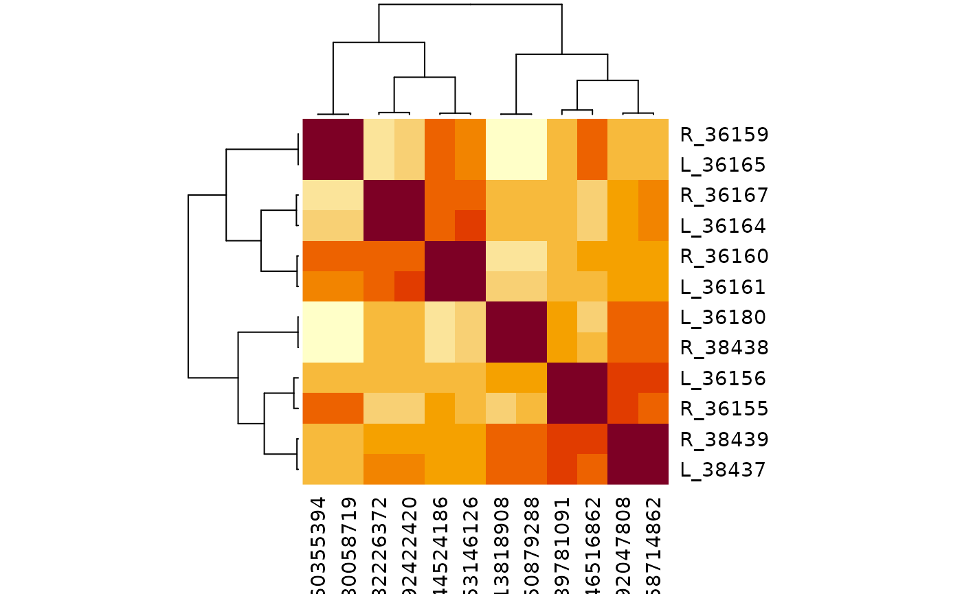

Cluster by predicted group

cf_cosine_plot(x, group = "pgroup", labRow = "{side}_{serial_id}")
#> Warning in coconat::partner_summary2adjacency_matrix(x[["outputs"]], inputcol =
#> "pre_key", : Dropping: 1088/1715 neurons representing 11404/29629 synapses due
#> to missing ids!
#> Warning in coconat::partner_summary2adjacency_matrix(x[["inputs"]], inputcol =
#> groupcol, : Dropping: 4256/4477 neurons representing 49876/59474 synapses due
#> to missing ids!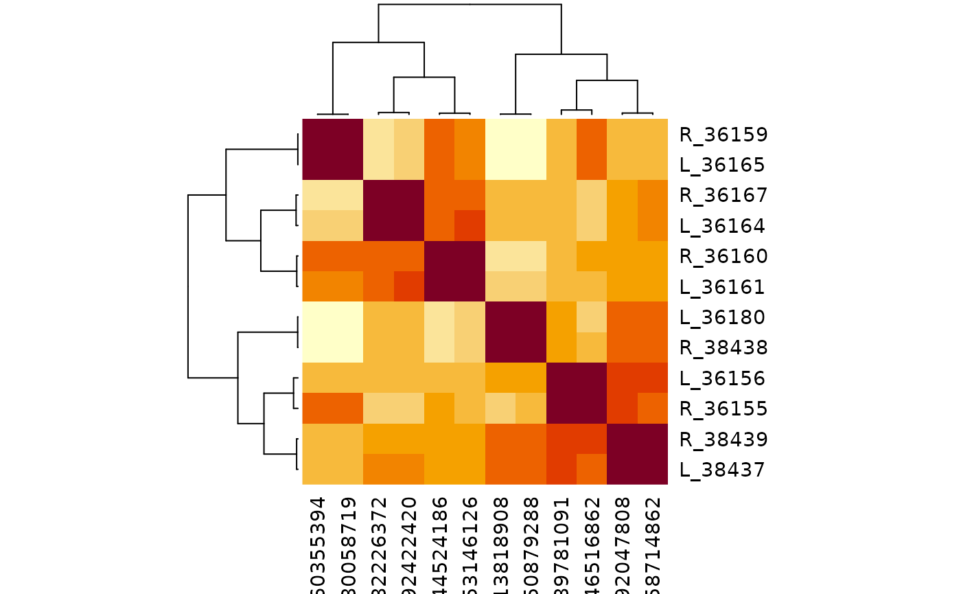

At the time of writing (September 2026) both groupings split the 12 neurons into six left/right pairs, which is reassuring. With pgroup the extra partner information gave a crisper result: 36155/36156 and 38437/38439 separated cleanly into two pairs rather than forming one loosely resolved cluster of four.

How the predicted group is defined

aedes_predict_group() returns ids that all live in the serial_id namespace, taking the first of these that is available:

type: the smallest serial_id among neurons of that type (a trailing ? is ignored, as are uninformative types listed in badtypes).
group: the curated group.
nblast_group: clusters of the form CNNNNN or NNNNN, where NNNNN is the smallest serial_id in the cluster (surrounding whitespace and a trailing ? are ignored). Any other value is ignored, so a bad cluster can be struck out by prefixing it with X (e.g. XC12345) without deleting the information.

Neurons with none of these get NA and are dropped as partners. With singletons = TRUE they instead fall back to their own serial_id, i.e. a group of one, so that every partner in FlyTable keeps its connectivity as a feature, behaving like group = FALSE for that neuron. This is off by default because a singleton partner can only be shared by neurons on the same side of the brain, which tends to pull left/right homologues apart.

Because type-derived ids use the smallest serial_id among the rows supplied, they can depend on which neurons are in the table. Within one cf_cosine_plot() call the partner metadata for each direction is fetched together, so the ids are consistent where it matters.

You can also compute predicted groups yourself, e.g. to use a custom badtypes list:

x$pgroup2 <- aedes_predict_group(x, badtypes = c(NA, "", "undefined"))
cf_cosine_plot(x, group = "pgroup2", labRow = "{side}_{serial_id}")
#> Warning in coconat::partner_summary2adjacency_matrix(x[["outputs"]], inputcol =
#> "pre_key", : Dropping: 1088/1715 neurons representing 11404/29629 synapses due
#> to missing ids!
#> Warning in coconat::partner_summary2adjacency_matrix(x[["inputs"]], inputcol =
#> groupcol, : Dropping: 4256/4477 neurons representing 49876/59474 synapses due
#> to missing ids!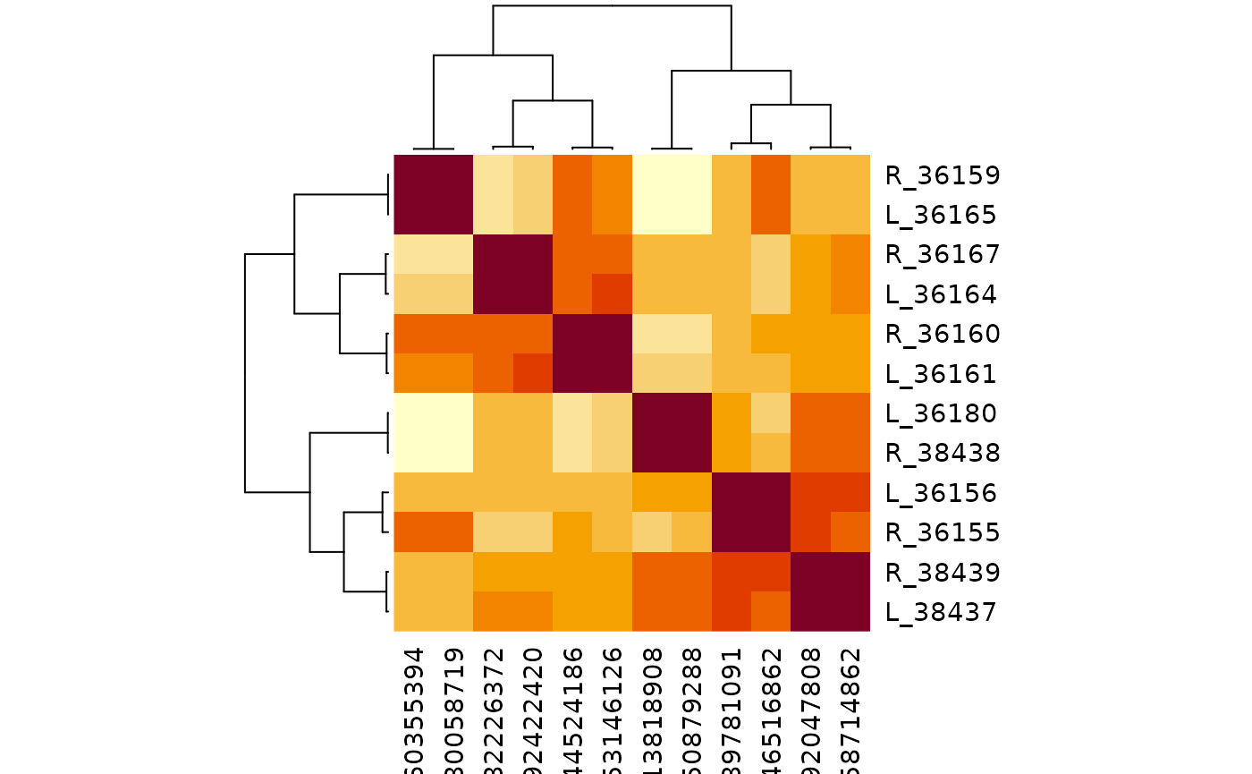

Rerunning this vignette

The results above depend on the live FlyTable annotations and CAVE connectivity, so they will change as proofreading and annotation progress.

Website. The pkgdown GitHub Actions workflow has the necessary FlyTable and CAVE credentials and evaluates this vignette in full whenever the site is rebuilt and deploys it on every push to main (pull requests also build the site, but do not deploy it). To refresh it without a push, trigger the workflow manually from the repository’s Actions tab or with gh workflow run pkgdown.yaml.

Locally. With FlyTable and CAVE access set up, render the vignette with the live chunks enabled:

Sys.setenv(AEDES_LIVE_VIGNETTES = "true")
rmarkdown::render("vignettes/connectivity-clustering.Rmd")

Saved results. When not evaluated live (e.g. during R CMD check or vignette("connectivity-clustering") from an installed package) the saved figures in vignettes/figures/ are shown. To refresh them, also set AEDES_SAVE_VIGNETTE_FIGURES=true when rendering locally, then update the saved coverage table and the “at the time of writing” text to match.